IMDB Movie Reviews

Here, we train a network to classify IMDB movie reviews as positive/negative !

A Binary Classification Example

Loading IMDB Dataset

The IMDB dataset has 50,000 highly polarized movie reviews. We use 25,000 reviews for training and 25,000 reviews for testing. Half of these 25,000 are positive and other half are negative reviews. These reviews (sequences of words) have been “pre-processed” i.e. turned into sequences of integers, where each integer stands for a specific word in a dictionary.

We use the top 10,000 most frequently occurring words by specifying num_words = 10,000. Instead of assigning individually, we use the %<-% which is the multi-assignment operator.

Code

library(keras)

imbd = dataset_imdb(num_words = 10000)

c(c(train_data, train_labels),c(test_data, test_labels)) %<-% imbd 

• The variables train_data and test_data are lists of reviews; each review is a list of word indices (encoding a sequence of words).
• The train_labels and test_labels are list of 0s and 1s, where 0 = negative and 1 = positive

Glimpse into our Data

Sample Reviews	Sentiment
This show was an amazing, fresh & innovative idea in the 70’s when it first aired. The first 7 or 8 years were brilliant, but things dropped off after that.	Negative
If you like original gut wrenching laughter you will like this movie. If you are young or old then you will love this movie, hell even my mom liked it. Great Camp!!!	Positive
This a fantastic movie of three prisoners who become famous. One of the actors is george clooney and I’m not a fan but this roll is not bad. Another good thing about the movie is the soundtrack (The man of constant sorrow). I recommand this movie to everybody. Greetings Bart	Positive
I have seen this film at least 100 times and I am still excited by it, the acting is perfect and the romance between Joe and Jean keeps me on the edge of my seat, plus I still think Bryan Brown is the tops. Brilliant Film.	Positive
I saw this movie in the middle of the night, when I was flipping through the channels and there was nothing else on to watch. It’s one of those films where you stop to see what it is - just for a moment! - but realize after twenty minutes or so that you just can’t turn it off, no matter how bad it is.	Negative

Data Preparation

We cannot feed lists of integers into a neural network. We have to turn these lists into tensors.

Encoding the integer sequences into a binary matrix -

Code

vectorize_sequences = function(sequences, dimension=10000){
  # create a empty-matrix of shape (length(sequences),dimensions)
  results = matrix(0, nrow=length(sequences),ncol=dimension) 
  # Set specific indices of results[i] to 1s
  for (i in 1:length(sequences)) results[i, sequences[[i]]] <- 1 
  results
}

x_train = vectorize_sequences(train_data)
x_test = vectorize_sequences(test_data)
str(train_data[[1]]) # int [1:218]
str(x_train[1,])     # num [1:10000]

# labels from integer to numeric
y_train = as.numeric(train_labels)
y_test = as.numeric(test_labels)
str(y_train) # num [1:25000]
str(y_test)  # num [1:25000]

Network Structure

So we have input data as a vector and labels as scalar (1s and 0s). Now, we can feed it to our neural network.

Code

library(keras)
library(dplyr)
model = keras_model_sequential() %>%
  layer_dense(units = 16, activation = "relu",input_shape = c(10000)) %>%
  layer_dense(units = 16, activation = "relu") %>%
  layer_dense(units = 1, activation = "sigmoid")

• 1st layer has 16 neurons which receives input vector of shape 10,000.

• 2nd layer has 16 neurons and is connected to all the neurons of the first layer. It uses a ReLU Activation function.

• 3rd layer is the output layer with 1 neuron and Sigmoid activation.

• Sigmoid activation gives us the probability whether a review is positive or negative.

Compile

Let’s see the other ways to configure the compilation step. We can specify the learning_rate to be used. Learning rate controls the speed with which the loss function is minimized.

Code

# specifying learning rate
model %>% 
  compile(optimizer = optimizer_rmsprop(learning_rate = 0.001), 
          loss="binary_crossentropy",
          metrics = c("accuracy"))
# specifying loss and metrics
model %>% compile(optimizer = optimizer_rmsprop(learning_rate =0.001), 
                  loss=loss_binary_crossentropy,
                  metrics = metric_binary_accuracy)
# finally using the default
model %>% compile(optimizer = "rmsprop", 
                  loss="binary_crossentropy",
                  metrics = c("accuracy"))

Creating Validation

Let’s create a Validation dataset where we set apart 10,000 samples from the original training data. This will be used adjust the hyper-parameters, spot over-fitting and improve our model’s performance.

Code

val_indices = 1:10000

x_val = x_train[val_indices,]
y_val = y_train[val_indices]

partial_x_train = x_train[-val_indices,]
partial_y_train = y_train[-val_indices]

Training

We train the model for 20 epochs in mini-batches of 512 samples - while monitoring loss and accuracy on 10,000 samples that we set apart.

Code

history = model %>% fit(partial_x_train, partial_y_train, 
                        epochs = 20, batch_size = 512,
                        validation_data = list(x_val, y_val))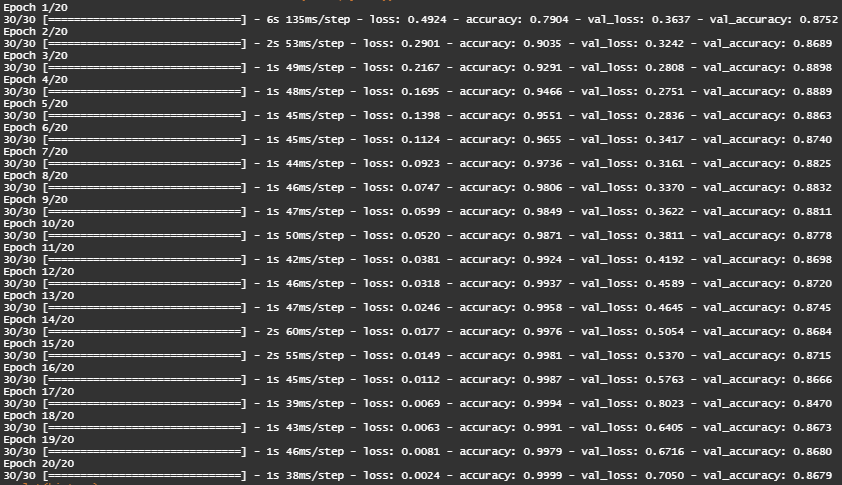

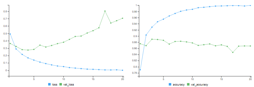
Training Results

Training Accuracy Plots

The Training Loss decreases with every epoch, and the training accuracy increases with every epoch. That’s what we expect when we run a gradient-descent optimization - the quantity we’re trying to minimize should be less with every iteration. But this isn’t the case for the validation loss and accuracy - they seem to peak at the 4th epoch - overfitting after 2nd epoch.

To prevent overfitting we must stop training after 3 epochs.

Code

model %>% fit(x_train, y_train, epochs=4,batch_size=512) 
# training accuracy = 92.63%
results = model %>% evaluate(x_test, y_test) 
# test accuracy = 87.57%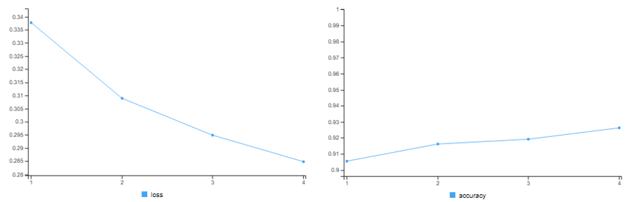

Training Accuracy Plots

This is a fairly naive approach which achieves an accuracy of about 85-86%

Predictions

Code

pred1 = model %>% predict(x_test[1:10,])

result1 = ifelse(pred1 >= 0.5, '1','0')
## likelihood of reviews being positive
# [1,] 0.10723257 (neg)
# [2,] 0.99999601
# [3,] 0.97627145
# [4,] 0.87328637
# [5,] 0.98664981
# [6,] 0.97016704
# [7,] 0.99999505
# [8,] 0.02466767 (neg)
# [9,] 0.99340731
#[10,] 0.99851567

test_labels[1:10]  # 0 1 1 0 1 1 1 0 0 1
as.numeric(result) # 0 1 1 1 1 1 1 0 1 1

As you can see, the network is confident for some samples (0.99 or more, or 0.01 or less) but less confident for others (0.7, 0.2)

Optimisation vs. Generalisation

• “Optimisation” deals with how well the model performs on training data.

• “Generalisation” deals with how well the model performs on test data (i.e. data it has never seen before)

When training begins, the training and testing loss are both low - here the model is underfitting because it has just started recognising the underlying patterns. Here, we can say that generalisation and optimization are correlated.

After some iterations, if generalisation stops improving - here the model is overfitting because it is learning patterns specific to training data which are irrelevant when it comes to new data. The process of dealing with overfitting is called “Regularisation”.

Dealing with Overfitting

1. Increase Training Data : using more data for training increases chances of better generalisation.

2. Reduce Network Size : i.e. the number of learnable parameters.

3. Adding Weight Regularisation : i.e. put constraints on the complexity of a network by forcing its weights to take only small values, which makes the distribution of weight values more regular. This is called weight-regularisation. here we add a cost to the loss function of the network - cost increases loss if weights are large.

   1. L1 regularisation - here the cost added is proportional to absolute value of weight coefficients.

   2. L2 regularisation - here the cost added is proportional to square of value of weight coefficients.

4. Dropout : A fraction of the features are zeroed out. 0.2 < dropout rate < 0.5 usually. During testing, no units are dropped out, the layer’s output values are scaled down by a factor equal to the dropout rate. On every iteration, we dropout different sets of 50% neurons.

Structural Experimenting

Model	Description	Training	Validation	Testing
Model 1	1 Layer with 16 Nodes	99.65%	87.20%	-
Model 2	3 Layers with 16 Nodes each	99.68%	86.84%	-
Model 3	3 Layers with (64,32,16) Nodes	99.16%	-	86.5%
Model 4	2 Layers with (16,16) Nodes with L1 Regularizer	89.49%	87.44%	87.1%
Model 5	2 Layers with (16,16) Nodes with L2 Regularizer	96.99%	87.19%	86.07%
Model 6	2 Layers with (16,16) Nodes with L1-&-L2 Regularizer	88.66%	83.07%	83.3%
Model 7	2 Layers with (16,16) Nodes with 50% Dropout Layer	97.83%	88.18%	87.3%

Model 1

Only 1 Hidden Layer

Here, we just use 1 hidden layer with 16 neurons.

Code

model.hidden1 = keras_model_sequential() %>%
  layer_dense(units = 16, activation = "relu",input_shape = c(10000)) %>%
  layer_dense(units = 1, activation = "sigmoid")

model.hidden1 %>% compile(optimizer = "rmsprop", 
                          loss="binary_crossentropy",
                          metrics = c("accuracy"))

history.hidden1 = model.hidden1 %>% 
  fit(partial_x_train, partial_y_train, 
      epochs = 20,batch_size = 512, 
      validation_data = list(x_val, y_val)) 

# training accuracy = 99.65% # validation accuracy = 87.20%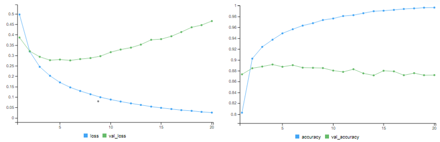

Training Accuracy Graphs

Clearly, the model with 1 hidden layer starts overfitting after first few epochs!

Model 2

Using 3 Hidden Layers

Here, we use 3 Hidden Layers with 16 neurons each.

Code

model.hidden3 = keras_model_sequential() %>%
  layer_dense(units = 16, activation = "relu",input_shape = c(10000)) %>%
  layer_dense(units = 16, activation = "relu") %>%
  layer_dense(units = 16, activation = "relu") %>%
  layer_dense(units = 1, activation = "sigmoid")

model.hidden3 %>% compile(optimizer = "rmsprop", 
                          loss="binary_crossentropy",
                          metrics = c("accuracy"))

history.hidden3 = model.hidden3 %>% 
  fit(partial_x_train, partial_y_train, 
      epochs = 20,batch_size = 512, 
      validation_data = list(x_val, y_val)) 

# training accuracy = 99.68% # validation accuracy = 86.84%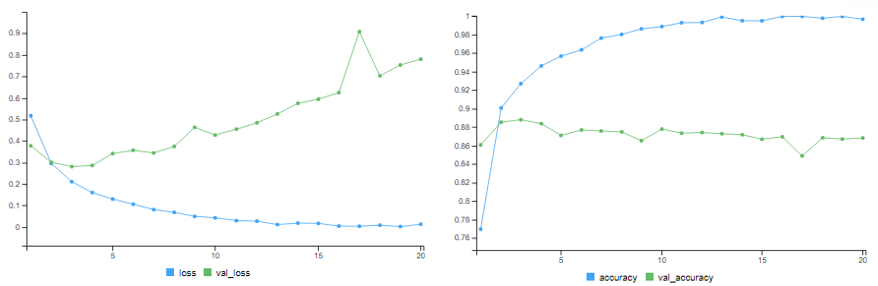

Training Accuracy Graphs

The training accuracy improves. But it starts overfitting after a few epochs.

Model 3

Using 3 Hidden Layers with different Configurations

Here, we change the number of neurons in the hidden layers to 64, 32 and 16 respectively.

Code

# hidden nodes (64, 32, 16) # epochs = 10
model.hidden3a = keras_model_sequential() %>%
  layer_dense(units = 64, activation = "relu",input_shape = c(10000)) %>%
  layer_dense(units = 32, activation = "relu") %>%
  layer_dense(units = 16, activation = "relu") %>%
  layer_dense(units = 1, activation = "sigmoid")

model.hidden3a %>% compile(optimizer = "rmsprop", 
                           loss="binary_crossentropy",
                           metrics = c("accuracy"))

history.hidden3a = model.hidden3a %>% 
  fit(x_train, y_train, epochs=10,batch_size=512) # training accuracy = 99.16%

results3a = model.hidden3a %>% evaluate(x_test, y_test) # test accuracy = 86.5%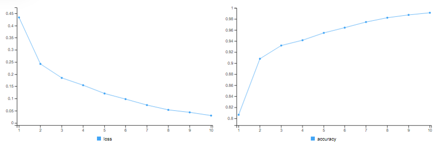

Training Accuracy Graphs

This model barely outperforms the initial model !

Model 4

Adding L1 Weight Regularisation

Code

model = keras_model_sequential() %>%
  layer_dense(units = 16, activation = "relu",input_shape = c(10000),
              kernel_regularizer = regularizer_l1(0.001)) %>%
  layer_dense(units = 16, activation = "relu",
              kernel_regularizer = regularizer_l1(0.001)) %>%
  layer_dense(units = 1, activation = "sigmoid")

model %>% compile(optimizer = "rmsprop", 
                  loss="binary_crossentropy",
                  metrics = c("accuracy"))

history = model %>% fit(partial_x_train, partial_y_train, 
                        epochs = 20, batch_size = 512, 
                        validation_data=list(x_val, y_val))
# training accuracy = 89.49% # validation accuracy = 87.44%

results = model %>% evaluate(x_test, y_test) # test accuracy = 87.1%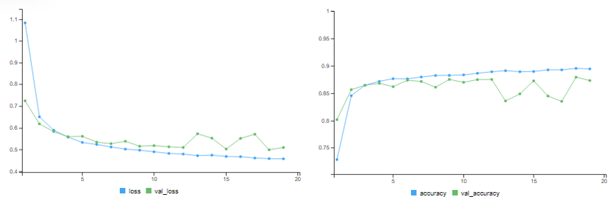

Training Accuracy Graphs

Model 5

Adding L2 Weight Regularisation

Code

model = keras_model_sequential() %>%
          layer_dense(units = 16, activation = "relu",input_shape = c(10000),
                      kernel_regularizer = regularizer_l2(0.001)) %>%
          layer_dense(units = 16, activation = "relu", 
                      kernel_regularizer = regularizer_l2(0.001)) %>%
          layer_dense(units = 1, activation = "sigmoid")

model %>% compile(optimizer = "rmsprop", loss="binary_crossentropy",
                  metrics = c("accuracy"))

history = model %>% fit(partial_x_train, partial_y_train, 
                        epochs=20, batch_size=512, 
                        validation_data=list(x_val, y_val))
# training accuracy = 96.99% # validation accuracy = 87.19%
results = model %>% evaluate(x_test, y_test) # test accuracy = 86.07%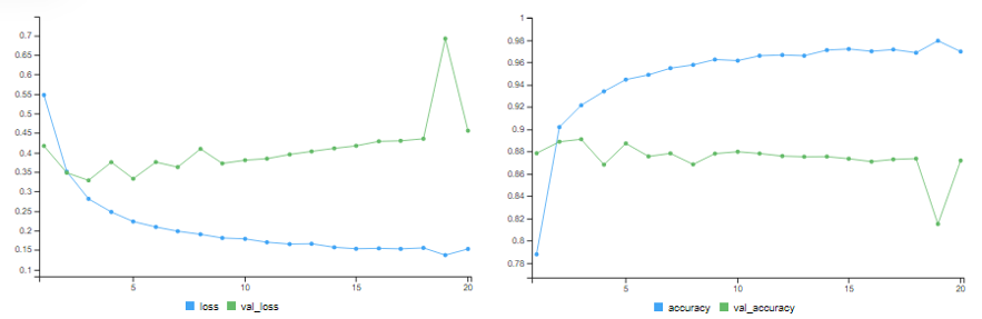

Training Accuracy Graphs

Model 6

Adding L1 & L2 Weight Regularisation

Code

model = keras_model_sequential() %>%
  layer_dense(units = 16, activation = "relu",input_shape = c(10000),
              kernel_regularizer = regularizer_l1_l2(l1 = 0.001,l2 = 0.001)) %>%
  layer_dense(units = 16, activation = "relu", 
              kernel_regularizer = regularizer_l1_l2(l1 = 0.001,l2 = 0.001)) %>%
  layer_dense(units = 1, activation = "sigmoid")

model %>% compile(optimizer = "rmsprop", loss="binary_crossentropy",
                  metrics = c("accuracy"))

history = model %>% fit(partial_x_train, partial_y_train, 
                        epochs=20,batch_size=512, 
                        validation_data=list(x_val, y_val))
# training accuracy = 88.66% # validation accuracy = 83.07%
results = model %>% evaluate(x_test, y_test) # test accuracy = 83.3%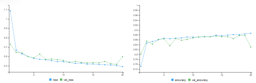

Training Accuracy Graphs

Model 7

Adding Dropout Layer

Code

model = keras_model_sequential() %>% 
  layer_dense(units = 16, activation = "relu",input_shape = c(10000)) %>%
  layer_dropout(rate = 0.5) %>%
  layer_dense(units = 16, activation = "relu") %>%
  layer_dropout(rate = 0.5) %>%
  layer_dense(units = 1, activation = "sigmoid")

model %>% compile(optimizer = "rmsprop", 
                  loss="binary_crossentropy",
                  metrics = c("accuracy"))

history = model %>% fit(partial_x_train, partial_y_train, 
                        epochs=20, batch_size=512, 
                        validation_data=list(x_val, y_val))
# training accuracy = 97.83% # validation accuracy = 88.18%

results = model %>% evaluate(x_test, y_test) # test accuracy = 87.3%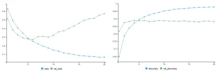

Training Accuracy Graphs

Final Model

For the Final Model we use both a Dropout Layer with L2 Weight Regularisation.

Code

model = keras_model_sequential() %>% 
  layer_dense(units = 32, activation = "relu",input_shape = c(10000),
              kernel_regularizer = regularizer_l2(0.001)) %>% 
  layer_dropout(rate = 0.5) %>% 
  layer_dense(units = 16, activation = "relu", 
              kernel_regularizer = regularizer_l2(0.001)) %>% 
  layer_dropout(rate = 0.5) %>% 
  layer_dense(units = 1, activation = "sigmoid")

model %>% compile(optimizer = "rmsprop", 
                  loss="binary_crossentropy",
                  metrics = c("accuracy"))

history = model %>% fit(x_train, y_train, epochs=4,batch_size=512) 
# training accuracy = 89.36%

results = model %>% evaluate(x_test, y_test) 
# test accuracy = 88.1%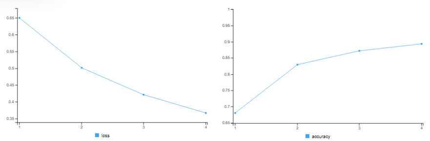

Training Accuracy Graphs

Model	Description	Training	Validation	Test
Final	2 Layers with (32,16) Nodes with 50% Dropout Layer & L2 regularizer	89.36%	-	88.1%

Evaluation & Prediction

Code

preds = model %>% predict(x_test[1:10,])

result = ifelse(preds >= 0.5, '1','0')
## likelihood of reviews being positive
# [1,] 0.2701703 (neg)
# [2,] 0.9999368
# [3,] 0.9951414
# [4,] 0.9118133
# [5,] 0.9855483
# [6,] 0.9277689
# [7,] 0.9999502
# [8,] 0.1525491 (neg)
# [9,] 0.9903402
#[10,] 0.9959549

# 1st and 8th reviews are negative
# remaining are positive

test_labels[1:10]  # 0 1 1 0 1 1 1 0 0 1
as.numeric(result) # 0 1 1 1 1 1 1 0 1 1

On comparing the 1st 10 predictions with actual values, we can see that the 4th and 9th reviews have been mis-classified as being positive when in reality they were negative.